ULink 2022 Genotype x OA Growth Analysis
research 03 Aug 2022Overview
Here I review the growth we have observed in our experiment. The total growth was less than we anticipated, but we still produced enough new skeleton with significant differences in growth rates and sensitivities to proceed forward with most of our tests.
Treatment Conditions
Labview Data
Figure 1. 10-minute averaged ERL Log
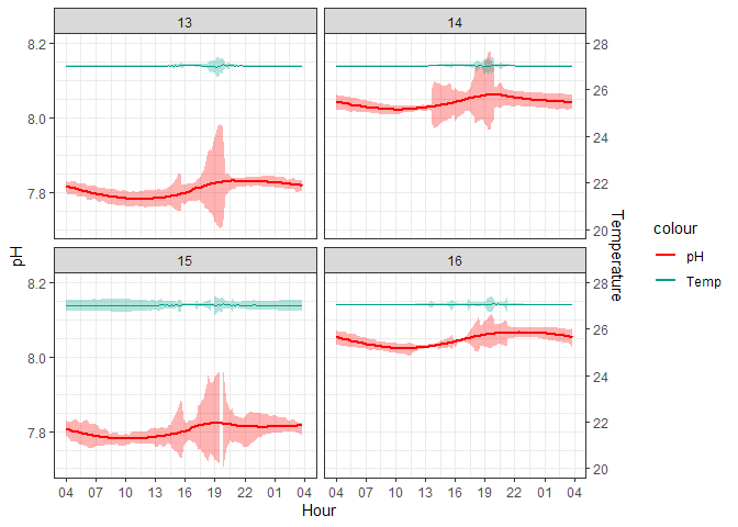
The peaks in the standard deviation are almost certainly caused by aquarium cleaning days when corals are removed into a separate bath and the sensors are capped causing logging errors. CO2 injection is turned off during these times so the aquariums themselves are not experiencing the conditions that the logged data are suggesting. The following graph filters out these spiked values which were programmatically identified by occurring during scheduled cleaning times and affecting multiple aquariums at once since cleaning occurred at the same time for all aquariums.
Figure 2. Cleaned 10-minute Averaged ERL Log
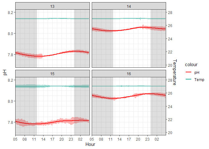
Variability is still present, but the extreme spikes caused by cleaning have been removed. Thus, any variability that remains is due to durafet error or experimental variability that affected the corals. For example, the durafet for T15 had much higher variability than the other aquariums. However, I believe this to be negligible as values are not spiking out of the treatment groups.
Carbonate Chemistry Data
500mL water samples were collected every Tuesday for analysis of the complete carbonate chemistry suite.
Time of Day
The bottles were not taken at exactly the same time of day (my fault). Therefore there will be enhanced variability of these stats since our diel variability is in action.
Figure 3. Times of Aquarium Bottle Sampling
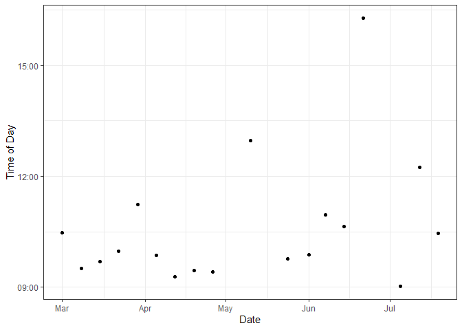
Sampling time had a mean of around 10a. 3 sampling times were taken after 12p with one sampling time around 4:20p
Carb Parameters
| tank | temp | TA | DIC | pCO2 | omega |
|---|---|---|---|---|---|
| T13 | 27.05 ± 0.02 | 2301.01 ± 21.14 | 2126.64 ± 22.78 | 835.70 ± 36.22 | 2.19 ± 0.07 |
| T14 | 27.05 ± 0.02 | 2300.12 ± 21.34 | 2000.13 ± 21.73 | 426.93 ± 14.74 | 3.46 ± 0.08 |
| T15 | 27.04 ± 0.02 | 2303.84 ± 21.56 | 2119.24 ± 24.84 | 848.20 ± 99.62 | 2.31 ± 0.18 |
| T16 | 27.07 ± 0.02 | 2297.52 ± 21.47 | 2004.24 ± 23.57 | 442.12 ± 17.83 | 3.38 ± 0.08 |
Statistics
| parameter | term | df | sumsq | meansq | statistic | p.value | significance |
|---|---|---|---|---|---|---|---|
| temp | treatment | 1 | 0.003 | 0.003 | 1.007 | 0.321 | NS |
| temp | treatment:tank | 2 | 0.004 | 0.002 | 0.636 | 0.534 | NS |
| temp | Residuals | 48 | 0.167 | 0.003 | NA | NA | NS |
| TA | treatment | 1 | 169.020 | 169.020 | 0.028 | 0.867 | NS |
| TA | treatment:tank | 2 | 96.270 | 48.135 | 0.008 | 0.992 | NS |
| TA | Residuals | 48 | 285247.509 | 5942.656 | NA | NA | NS |
| DIC | treatment | 1 | 189577.501 | 189577.501 | 26.960 | 0.000 | xxx |
| DIC | treatment:tank | 2 | 465.459 | 232.730 | 0.033 | 0.967 | NS |
| DIC | Residuals | 48 | 337526.642 | 7031.805 | NA | NA | NS |
| pCO2 | treatment | 1 | 2157966.567 | 2157966.567 | 56.404 | 0.000 | xxx |
| pCO2 | treatment:tank | 2 | 2513.434 | 1256.717 | 0.033 | 0.968 | NS |
| pCO2 | Residuals | 48 | 1836441.545 | 38259.199 | NA | NA | NS |
| omega | treatment | 1 | 17.735 | 17.735 | 109.739 | 0.000 | xxx |
| omega | treatment:tank | 2 | 0.135 | 0.068 | 0.418 | 0.661 | NS |
| omega | Residuals | 48 | 7.757 | 0.162 | NA | NA | NS |
Temperature and total alkalinity were not significantly different between treatments or within treatments (p>>0.05). DIC, pCO2, and \(\Omega_{Ar}\) (p<0.001) were significantly different between treatment, but not between aquariums within treatment (p>>0.05). In other words, our system reproducibly altered the carbonate chemistry parameters with high precision.
Calcification Analysis
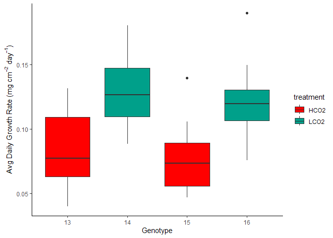
Figure 4. Avg Daily Growth by (A) Treatment and (B) Genotype
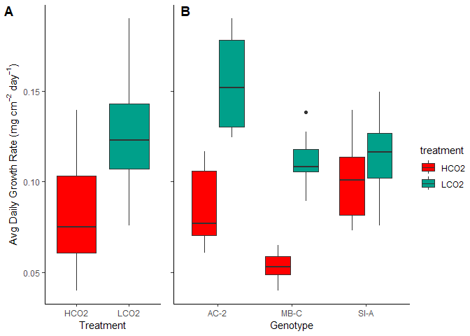
| treatment | n | mean | sd |
|---|---|---|---|
| HCO2 | 37 | 0.081 | 0.027 |
| LCO2 | 37 | 0.126 | 0.028 |
| .y. | group1 | group2 | n1 | n2 | statistic | df | p | p.signif |
|---|---|---|---|---|---|---|---|---|
| G | HCO2 | LCO2 | 37 | 37 | -7.0659 | 72 | 0 | \*\*\*\* |
| .y. | group1 | group2 | effsize | n1 | n2 | magnitude |
|---|---|---|---|---|---|---|
| G | HCO2 | LCO2 | -1.6428 | 37 | 37 | large |
| term | contrast | adj.p.value | significance |
|---|---|---|---|
| treatment | LCO2-HCO2 | 0.0000 | xxx |
| treatment:genotype | LCO2:AC-2-HCO2:AC-2 | 0.0000 | xxx |
| treatment:genotype | LCO2:MB-C-HCO2:MB-C | 0.0000 | xxx |
| genotype | SI-A-MB-C | 0.0001 | xxx |
| genotype | SI-A-AC-2 | 0.1385 | NS |
| treatment:genotype | LCO2:SI-A-HCO2:SI-A | 0.4558 | NS |
The mean calcification rate in the HCO2 group was mean 0.081 (SD = 0.027) mg/ \(cm^2\) /day, whereas the mean in the LCO2 group was 0.126 (SD = 0.028). A Student two-samples t-test showed that the difference was statistically significant, t(72) = -7.066, p < 0.0001, d = -1.643. Thus, the ocean acidification group saw on average a 36% reduction in calcification rates. The effects, however, were not even across the genotypes (Table 5).
Tank Effects
We saw above that tank conditions were significantly different among treatment groups, but not individual aquariums within treatment. We also saw that calcification rates were significantly different among treatment groups. Here I am analyzing tank effects on the calcification rate and investigating if calcification rates were significantly different between aquariums within the same treatment group. This will dictate whether we need to include tank as a random intercept in our ANOVA models.
Figure 5. Avg Daily Growth by Tank and Treatment
Tank Effects Statistics
| treatment | .y. | group1 | group2 | n1 | n2 | statistic | df | p | p.adj | p.adj.signif |
|---|---|---|---|---|---|---|---|---|---|---|
| HCO2 | G | 13 | 15 | 19 | 18 | 0.991 | 34.650 | 0.329 | 0.329 | ns |
| LCO2 | G | 14 | 16 | 19 | 18 | 1.074 | 34.937 | 0.290 | 0.290 | ns |
No observable differences of mean calcification rate when comparing within treatment groups.
Mixed Effects Model
Here I created a mixed effects model model to account for the lack of independence brought upon by having multiple corals grown in the same tank and the possible tank-specific effects that may have affected calcification rates. Including this random effect increased the AIC from -354 to -352 as compared to a fixed-effects only model, and therefore I will not include random tank effects in my analysis.
As a reminder, here is the fixed effects model as shown above:
modFixed <- totalGrowth %>%
  aov(G ~ genotype*treatment, data=.)

modFixed %>%
  summary()
Df Sum Sq Mean Sq F value Pr(>F)
genotype 2 0.01374 0.00687 17.46 7.61e-07 * treatment 1 0.03956
0.03956 100.54 4.89e-15 *** genotype:treatment 2 0.01169 0.00584 14.85
4.46e-06 *** Residuals 68 0.02676 0.00039
— Signif. codes: 0 ‘’ 0.001 ’**’ 0.01 ’’ 0.05 ‘.’ 0.1 ’ ’ 1
Here is the mixed effects model with the tank identity set as a random factor to give each tank its own, random intercept. Notice, including the random effects decreases the absolute value of the AIC. Therefore, this new model better describes the data.
modRandom <- totalGrowth %>%
  lmerTest::lmer(G ~ genotype * treatment + (1|tank),
                 data=.)
modRandom %>%
  anova() %>%
  tidy() %>%
  kbl()
| term | sumsq | meansq | NumDF | DenDF | statistic | p.value |
|---|---|---|---|---|---|---|
| genotype | 0.0167813 | 0.0083906 | 2 | 66.206864 | 21.46841 | 0.0000001 |
| treatment | 0.0340982 | 0.0340982 | 1 | 2.012228 | 87.24428 | 0.0110507 |
| genotype:treatment | 0.0116516 | 0.0058258 | 2 | 66.206864 | 14.90602 | 0.0000045 |
#redefining modRandom w/ REML=F for AIC comparison
modRandom <- totalGrowth %>%
  lmerTest::lmer(G ~ genotype * treatment + (1|tank), REML = F,
                 data=.)

AIC(modFixed, modRandom) %>%
  kbl()
| df | AIC | |
|---|---|---|
| modFixed | 7 | -362.4413 |
| modRandom | 8 | -360.4413 |
Powder Available
Figure 6. Amount of New CaCO3 Precipitated
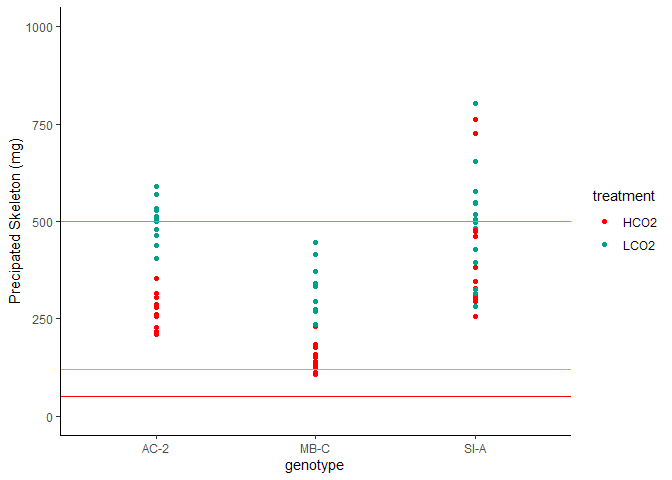
The amount of new aragonite precipated is visualized above. Horizontal lines denote thresholds for tests: >500mg = green (complete suite including XRD), >120 mg = orange (complete suite sans XRD), >50mg = red (TGA and isotope only).
Linear Extension
Figure 7. Avg Daily Linear Extension by Treatment
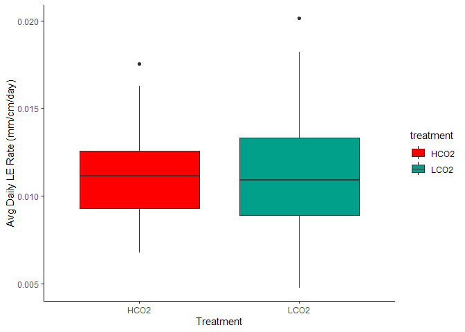
Figure 8. Avg Daily Linear Extension by Treatment and Aquarium
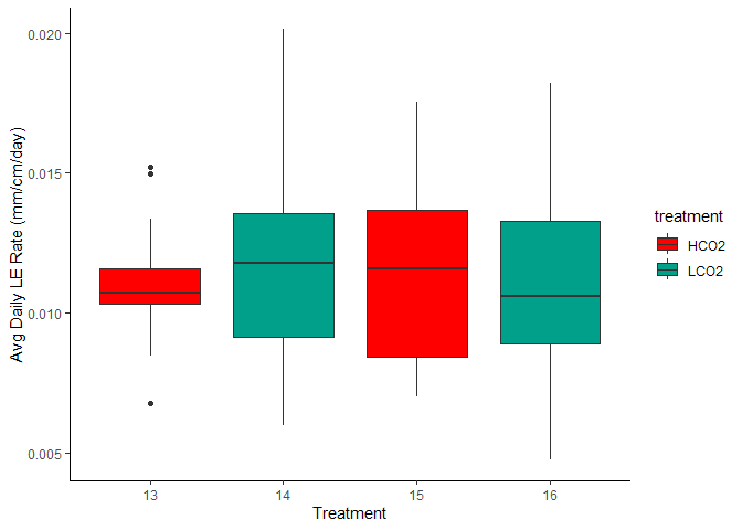
Figure 9. Avg Daily Linar Extension by Genotype and Treatment
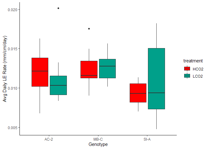
Such large variability in that SI-A ambient group.
| treatment | n | mean | sd |
|---|---|---|---|
| HCO2 | 37 | 0.011 | 0.003 |
| LCO2 | 36 | 0.012 | 0.004 |
| .y. | group1 | group2 | n1 | n2 | statistic | df | p | p.signif |
|---|---|---|---|---|---|---|---|---|
| prod | HCO2 | LCO2 | 37 | 36 | -0.4283 | 71 | 0.67 | ns |
| .y. | group1 | group2 | effsize | n1 | n2 | magnitude |
|---|---|---|---|---|---|---|
| prod | HCO2 | LCO2 | -0.1003 | 37 | 36 | negligible |
| term | contrast | adj.p.value | significance |
|---|---|---|---|
| genotype | SI-A-MB-C | 0.0218 | x |
| genotype | SI-A-AC-2 | 0.1599 | NS |
| treatment | LCO2-HCO2 | 0.6562 | NS |
| treatment:genotype | LCO2:SI-A-HCO2:SI-A | 0.6948 | NS |
| treatment:genotype | LCO2:AC-2-HCO2:AC-2 | 0.9697 | NS |
| treatment:genotype | LCO2:MB-C-HCO2:MB-C | 1.0000 | NS |
The mean linear extension rate in the HCO2 group was mean 0.011 (SD = 0.003) mm/cm/day, whereas the mean in the LCO2 group was 0.012 (SD = 0.004). A Student two-samples t-test showed that the difference was not statistically significant, t(71) = -0.428, p =0.124, d = -0.1.
Takeaways and Next Steps
Overall growth was less than hoped for. However, there is enough new skeleton for nearly all the powder tests that we want to conduct: FTIR, TGA, boron isotopes, and Raman.For nanoindentation tests, we should have enough new growth to run on a majority of samples.
Linear extension was measured by maximum vertical height as measured with calipers. We additionally have initial 3d scans of all corals and post 3d scans of a subset of 48 corals (n=3 per genotype per tank). From this data, we can extract surface area to volume ratios and see how this changed among genotypes and treatments. This analysis still needs to be done.
CT Scanning
The micro-ct scan is currently out of service. We can use the large ct-scanner to determine bulk density. The scanner has a resolution of 0.1mm/scan so we can measure the density of the new growth. This growth is isolated to the highly variable apical tips which may cause some problems. See this post which discusses the ct-scanning analysis of apical tips done on Langdon’s OA corals.