Preliminary Raman Analysis
research 05 Dec 2023Overview
Raman is a spectroscopic technique which measures inelastic light scattering due to vibrational energy within and between molecules. In practice, Raman can provide important information regarding the identification and chemical composition of minerals. It’s also proposed that Raman can derive the fluid characteristics from which a mineral was formed (DeCarlo et al 2017). As in all spectroscopy techniques, we are characterizing distinct peaks. For calcium carbonates, we are most interested in the v1 peak at ~1085 $cm^{-1}$ (some literature on CCA look at high-magnesium calcite v1 peak at 1089 $cm^{-1}$), which corresponds to the symmetric stretching of the carbonate C-O bond. The width of this v1 peak denotes higher disorder, which may correlate with supersaturated solutions and faster reaction kinetics (i.e. crystal formation).
Raman has successfully been used to describe biogenic calcium carbonates and mineralogical conformations under various perturbations. Kamenos et al. (2013) observed decreases in v1 peak width as ambient seawater pCO2 increased and further noticed marked decreases in peak width when the pCO2 was rapidly increased compared to a gradual increase in pCO2. Follow up work by this research team further supported this linear relationship between pCO2 concentration and v1 peak width in CCA cultured under multiple pCO2 scenarios, and they have since proposed Raman as a tool for paleoclimate reconstructions (Pauly et al. 2014).
Corals calcify from an internal fluid, which is composed of external seawater which has been altered to promote calcification. The differential modifications of this calcifying fluid by different coral species may explain the species-specific sensitivity to ocean acidification and has been an active area of research for over a decade. Recently, Tom DeCarlo has published numerous papers using Raman to characterize corals’ calcifying fluid aragonite saturation state. Given the background above, DeCarlo et al. (2017) built a regression of v1 FWHM of abiogenic aragonites precipitated at known aragonite saturation states in the lab. They have applied this logarithmic regression to calculate the calcifying fluid aragonite saturation state of corals from experiments culturing corals under temperature and CO2 stress and from field experiments, cores, and a thoroughly analyzed paleoclimate coral CRM (JCp-1). To highlight a few notable findings from their Raman work:
- They were able to identify diurnal, night-day patterns of increasing v1 FWHM ($\Omega_{cf}$) corresponding to light-enhanced calcification, highlighting the high spatial resolution available with Raman (DeCarlo et al. 2019);
- They combined Raman spectroscopy data with boron isotopes and elemental geochemistry to constrain calcium concentrations of the calcifying fluid. In Pocillopora damicornis cultured under high pCO2, they observed a nearly 25% increase in [$Ca_2$]cf and constant calcification rates. They propose increasing calcium concentrations of the calcifying fluid as an alternative mechanism to maintain aragonite saturation states despite decreasing carbonate concentrations (DeCarlo et al., 2018);
- They used Raman on live corals held in seawater filled containers, showcasing the ability to study corals in vivo (DeCarlo et al. 2019).
Recently, work by Kellock et al. (2022) have highlighted the role of organic content in modifying the FWHM of coral’s v1 peak, muddying the interpretation of FWHM as a proxy for coral calcification response to OA. Aspartic acid is the largest concentration of amino acids in coral skeletons, and the authors noticed that when concentrations ≥ 1mM were included in lab-created aragonite, there was a significant increase in the v1 FWHM.
All in all, Raman has a number of advantages compared to other biogeochemial tools commonly used to study coral calcification mechanisms including high spatial resolution, minimal sample preparation, non-destructive sampling, and ability to use Raman on live coral.
Nevertheless, there are some shortcomings of Raman. Raman is sensitive to fluoresence from organics (mitigated here by cleaning samples in buffered $H_2O_2$), Raman machines will each produce slightly different spectra, and quantitative analysis of Raman is influenced by spectral resolution, which itself is influenced by many factors intrinsic to different spectrometers and user-chosen parameters. We can overcome some of these shortcomings by using a daily peak position calibration and a peak width calibration of CRMs. Daily peak calibration is standard practice and was performed for all shown spectra. We will attempt to use JcP-1 as the aragonite peak-width calibration, since DeCarlo et al. published 440 spectra, which we can accept as the “standard/true” values.
Bibliography of Raman used for biogenic calcium carbonates
- Kamenos NA, Burdett HL, Aloisio E, Findlay HS, Martin S, Longbone C, Dunn J, Widdicombe S, Calosi P. 2013. Coralline algal structure is more sensitive to rate, rather than the magnitude, of ocean acidification. Global Change Biology. 19(12):3621–3628. https://doi.org/10.1111/gcb.12351
- Kamenos NA, Perna G, Gambi MC, Micheli F, Kroeker KJ. 2016. Coralline algae in a naturally acidified ecosystem persist by maintaining control of skeletal mineralogy and size. Proceedings of the Royal Society B: Biological Sciences. 283(1840):20161159. https://doi.org/10.1098/rspb.2016.1159
- Hennige SJ, Wicks LC, Kamenos NA, Perna G, Findlay HS, Roberts JM. 2015. Hidden impacts of ocean acidification to live and dead coral framework. Proceedings of the Royal Society B: Biological Sciences. 282(1813):20150990. https://doi.org/10.1098/rspb.2015.0990
- Pauly M, Kamenos NA, Donohue P, LeDrew E. 2015. Coralline algal Mg-O bond strength as a marine pCO2 proxy. Geology. 43(3):267–270. https://doi.org/10.1130/G36386.1
- DeCarlo TM, Ross CL, McCulloch M. 2019. Diurnal cycles of coral calcifying fluid aragonite saturation state. Marine Biology. 166(3):1–6. https://doi.org/10.1007/s00227-019-3468-6
- Decarlo TM, Comeau S, Cornwall CE, McCulloch MT. 2018. Coral resistance to ocean acidification linked to increased calcium at the site of calcification. Proceedings of the Royal Society B: Biological Sciences. 285(1878). https://doi.org/10.1098/rspb.2018.0564
- DeCarlo TM, Comeau S, Cornwall CE, Gajdzik L, Guagliardo P, Sadekov A, Thillainath EC, Trotter J, McCulloch M. 2019. Investigating marine bio‐calcification mechanisms in a changing ocean with in vivo and high‐resolution ex vivo Raman spectroscopy. Global Change Biology. 25(5):1877–1888. https://doi.org/10.1111/gcb.14579
- Kellock C, Castillo Alvarez MC, Finch A, Penkman K, Kröger R, Clog M, Allison N. 2022. Optimising a method for aragonite precipitation in simulated biogenic calcification media. PLoS One. 17(12):e0278627. https://doi.org/10.1371/journal.pone.0278627
Peak Identification
To ensure the collected Raman spectra were characteristic of aragonite, an extended peak of the entire region (0-4000 $cm^{-1}$) was collected once per sample on a haphazardly chosen grain. The following peak characteristics were identified:
- v1 peak @ ~1085 (calcium carbonate)
- v4 peak @ ~700-708 (aragonite), @ ~712 (calcite)
- double v4 peak (aragonite)
- v2 peak @ ~280 (calcite), 210 (aragonite)
Data Analysis
Raman peaks of solid samples can be closely approximated with a Gaussian curve, from which the peak area, full-width at half maximum (FWHM), and peak position can be easily extracted. DeCarlo et al. 2017 released R code which calculates a Gaussian curve and the three peak parameters for the v1 peak. Spectroscopy is commonly analyzed with proprietary software, such as Origin Pro, and I used this software and its standard operating protocols to compare to the DeCarlo method. Finally, I analyzed the data in a third, open-source way by modifying the DeCarlo routine and implementing similar data processing steps from the OpenSpecy package to closely approximate the Origin Pro Routine.
In summary, I analyzed the data in three ways,
- Modified DeCarlo Routine - SNV normalization (identical to Z-scores), create Gaussian curve
- Kiel Routine - subtract baseline with a 5th order polynomial, SNV normalization, create Gaussian curve
- Origin Pro Routine - subtract baseline with asymmetric least squares smoothing baseline, SNV normalization, create Gaussian curve
The only modification of the original DeCarlo Routine was the incorporation of an SNV normalization step to remove peak intensity artifacts and make spectra more comparable across Raman spectrometers. The Kiel Routine is identical to the Modified DeCarlo Routine, except it incorporates a baseline subtraction step.
There is a small difference in the Gaussian fit between the Origin Pro and the two open source scripting routines. Origin Pro uses this form of the Gaussian curve, $y = y_0 + ke ^\frac{-(x-p)^2}{2s^2}$ while the two open source scripting routines incorporate an m term, which corresponds to the slope of the background intensity $y = y_0 + mx + ke ^\frac{-(x-p)^2}{2s^2}$
where y is the intensity, $y_0$ is the background intensity, x is the Raman shift, m is the background slope, k is the peak height, p is the peak position (in Raman shift numbers), and s is the standard deviation. The FWHM of the Gaussian curve is calculated by, $FWHM = 2s\sqrt{2ln(2)}$ and the area of the Gaussian curve is calculated by, $A =1.064467\times FWHM \times \text{peak height}$. In R, a non-linear least squares approach is used to fit the Gaussian model to the measured intensity data.
When the baseline has been subtracted or in an otherwise cleaned spectra, m is approximately 0 and the two Gaussian forms are identical.
I did not smooth the data in any of these analysis routines as is customary for visualization purposes, since smoothing is not recommended for quantitative analysis unless absolutely necessary (due to random peaks, low SNR).
JCp-1 Results
Figure 1. Comparison of analysis routine for four peak parameters
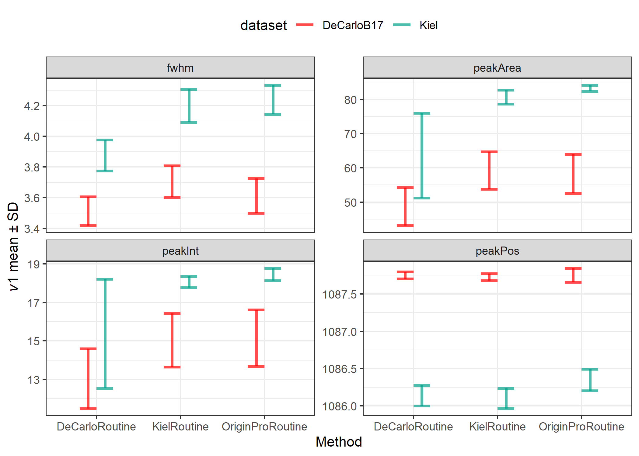
Table 1. Determinants for each method including coefficient of variation (%CV = precision), and relative standard error (%rse = precision, % accuracy, and systematic error correction
| metric | method | cv | rse | JcP1_accuracy | JcP1_sysCorrection |
|---|---|---|---|---|---|
| fwhm | DeCarloRoutine | 2.639 | 0.476 | 89.644 | 0.364 |
| fwhm | KielRoutine | 2.666 | 0.470 | 86.671 | 0.494 |
| fwhm | OriginProRoutine | 2.681 | 0.428 | 82.707 | 0.625 |
| peakArea | DeCarloRoutine | 15.411 | 3.350 | 69.475 | 14.872 |
| peakArea | KielRoutine | 5.862 | 0.623 | 63.867 | 21.415 |
| peakArea | OriginProRoutine | 5.413 | 0.400 | 57.223 | 24.935 |
| peakInt | DeCarloRoutine | 15.168 | 3.196 | 82.095 | 2.336 |
| peakInt | KielRoutine | 5.448 | 0.479 | 79.934 | 3.017 |
| peakInt | OriginProRoutine | 5.699 | 0.504 | 78.178 | 3.306 |
| peakPos | DeCarloRoutine | 0.009 | 0.002 | 99.852 | -1.610 |
| peakPos | KielRoutine | 0.008 | 0.002 | 99.851 | -1.625 |
| peakPos | OriginProRoutine | 0.011 | 0.002 | 99.871 | -1.402 |
The FWHM of the DeCarlo et al. (2017) spectra is consistently less than the FWHM we measured for the JcP-1 CRM, with a difference ranging between 0.364-0.625, which grants an accuracy of 89.6-82.7%. However, the precision of each analysis routine produces a comparable CV between 2.64-2.68%. There is a general increase in measured FWHM when using the Kiel routine and Origin Pro routine compared to the DeCarlo Routine regardless of dataset, while the difference between the Kiel Routine and the Origin Pro Routine are comparably small.
For peak area, the Kiel routine and Origin Pro routine produce comparable results with higher precision, 5.86% and 5.41%, but sacrifice accuracy, 63.87% and 57.22%, respectively compared to the DeCarlo routine, which has a precision of 15.41% and an accuracy of 69.48%.
For peak intensity, the DeCarlo routine had the greatest variability, with a precision of 15.1%. The accuracy’s were approximately comparable for all three methods, ranging from 78.2-82.1%. There was further variability in the DeCarlo dataset compared to the spectra we collected. The DeCarlo dataset also had on average less peak intensity than our measured peak intensity. A likely source for these dataset differences is the laser excitation energy. I measured data with the laser set to 100% intensity to maximize the signal to noise ratio, while the DeCarlo dataset was measured with a 1% intensity laser.
For peak position, all three methods had excellent accuracy and precision, with a positional difference of approximately 1.4 - 1.62 $cm^{-1}$ with a precision of approximately 0.01%.
There are two main points which need to be kept in mind when thinking of these accuracy and precision numbers. First, I only measured 10 spectra of JCp-1, while the DeCarlo dataset is comprised of 440 spectra (2-3 spectra are rejected due to poor spectral quality). Relative standard error (RSE) should be a better comparison of precision when the N varies significantly, but the conclusions remain the same when using RSE or CV in the table above. I plan to measure at least 10 spectra (will shoot for 25 going forward) during each Raman session to correct that day’s data. I will revisit this accuracy analysis and pool all measured spectra to compare against the DeCarlo dataset. Second, JCp-1 has been phased out of the biogeochemical community since there was large variability and it was deemed not sufficient for climate quality reconstructions of pH from coral. Thus, the biogeochemistry community has shifted to synthetic simulated coral standards, which has led to increased accuracy and inter-lab comparisons. This seems obvious since JCp-1 is a single large Porites colony that was collected from the wild and subsequently ground in a ball-mill to a homogenized powder. Thus a given aragonite grain from this homogenized sample may be compositionally distinct from another grain due to overall decreases in aragonite saturation state (OA effect), seasonal and daily changes in aragonite saturation state, sampling location within colony, etc.
Therefore, I am not choosing a routine method solely based on accuracy as the grains measured by DeCarlo may very well have different peak properties than the grains I am measuring. With an average cv across measurements of 3.49% and an average accuracy of 82.6%, I will proceed to use the Kiel Routine for all subsequent analyses. For comparison, the DeCarlo routine had an average cv of 8.3% and an average accuracy of 85.3%. Thus, I will subtract 0.494 from all FWHM measurements to enable the use of DeCarlo’s abiotic samples and aragonite saturation state curve.
Reanalysis of DeCarlo’s Abiotic Spectra
DeCarlo created abiogenic aragonite samples in the lab. These were then measured on a Raman spectrometer at Woods Hole for initial analysis, re-analyzed at the University of Westrn Australia (UWA), and then re-analyzed again at Hawaii Pacific Univeristy. I am going to ignore the Woods Hole measurements as these have not been extensively used for DeCarlo’s Raman work. The measurements and generated calibration curve at UWA have been extensively used. Further, the JcP measurements from above were all measured on the UWA setup. I am purposefully including the new Hawaii Pacific University measurements as it is nearly the exact same Renishaw Raman setup that is available at FIU in Dr. Prasad’s lab and was used for DeCarlo’s most recent publication.
The goal with this analysis is to recreate two calibration curves from these two datasets of DeCarlo’s abiotic aragonite using the Kiel Routine outlined above. I will then compare to the two published calibration curves. D17 denotes the published JCP1 and abiogenic spectra from DeCarlo et al. (2017) and MD23 denotes the abiogenic spectra from Mantanona & DeCarlo (2023).
Unfortunately MD23 did not measure the JCp-1 CRM, however, they did measure the same seven abiogenic aragonite grains, which is a more powerful correction than a single CRM. Here, we will align the MD23 measurements to the D17 measurements with both an OLS regression and an estimation of systematic error assuming the D17 measurements are the “true/standard” measurements (i.e. subtract a constant).
Violin (density plots) in Figure 2 show the spread of measured v1 FWHM of the abiogenic aragonite from the D17 and MD23 datasets. There is an average systematic error of error of 0.463, which is quite similar and within the estimate to our JCp-1 derived systematic error of 0.494. This gives me great confidence that the measurements on Dr. Prasad’s spectrometer closely approximate the measurements on Dr. DeCarlo’s spectrometer in Hawaii. These values both differ, however, from the values measured on the WITEC spectrometer at UWA. Alternatively we can use the OLS regression to fit the fwhm_MD23 to the values measured in D17 using the equation, MD23_fitted = 1.288 X MD23_raw - 1.745.
Figure 2. Violin plots of measured abiogenic aragonite FWHM in A D17 and B MD23. Dashed lines are published curves.
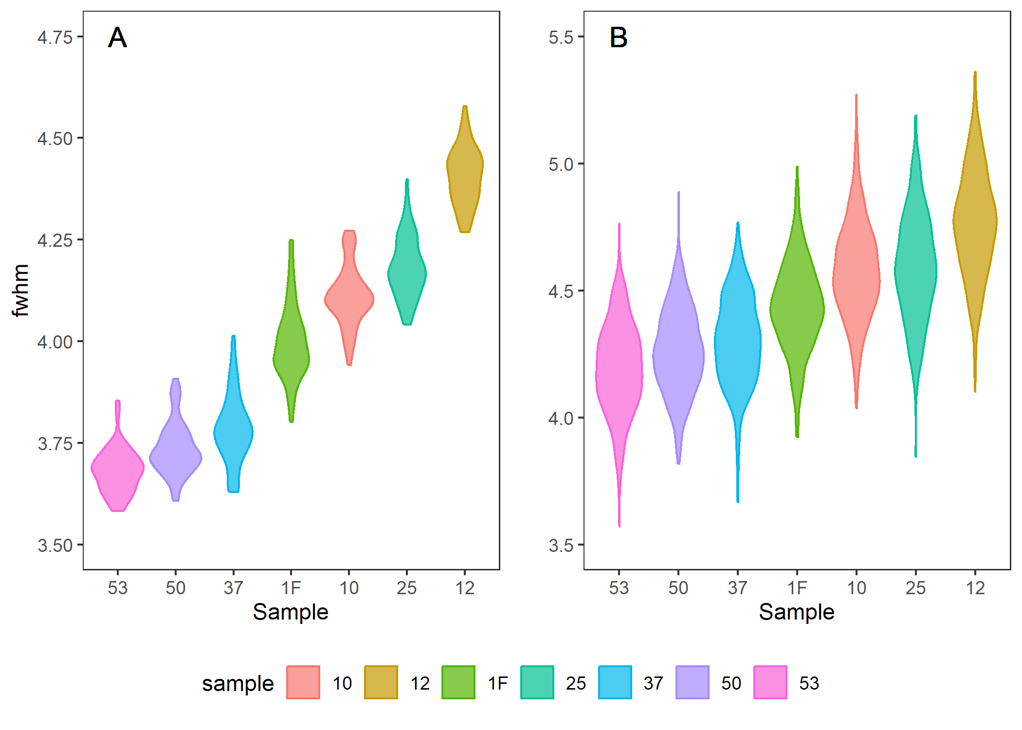
Table 2. FWHM means for the two datasets for each abiogenic sample along with the known aragonite saturation state
| sample | omega | fwhm_MD23 | fwhm_D17 | diff |
|---|---|---|---|---|
| 53 | 10 | 4.195 | 3.682 | 0.514 |
| 50 | 11 | 4.263 | 3.736 | 0.527 |
| 37 | 14 | 4.305 | 3.784 | 0.521 |
| 1F | 16 | 4.437 | 3.998 | 0.440 |
| 10 | 19 | 4.579 | 4.112 | 0.468 |
| 25 | 24 | 4.593 | 4.182 | 0.411 |
| 12 | 30 | 4.766 | 4.407 | 0.359 |
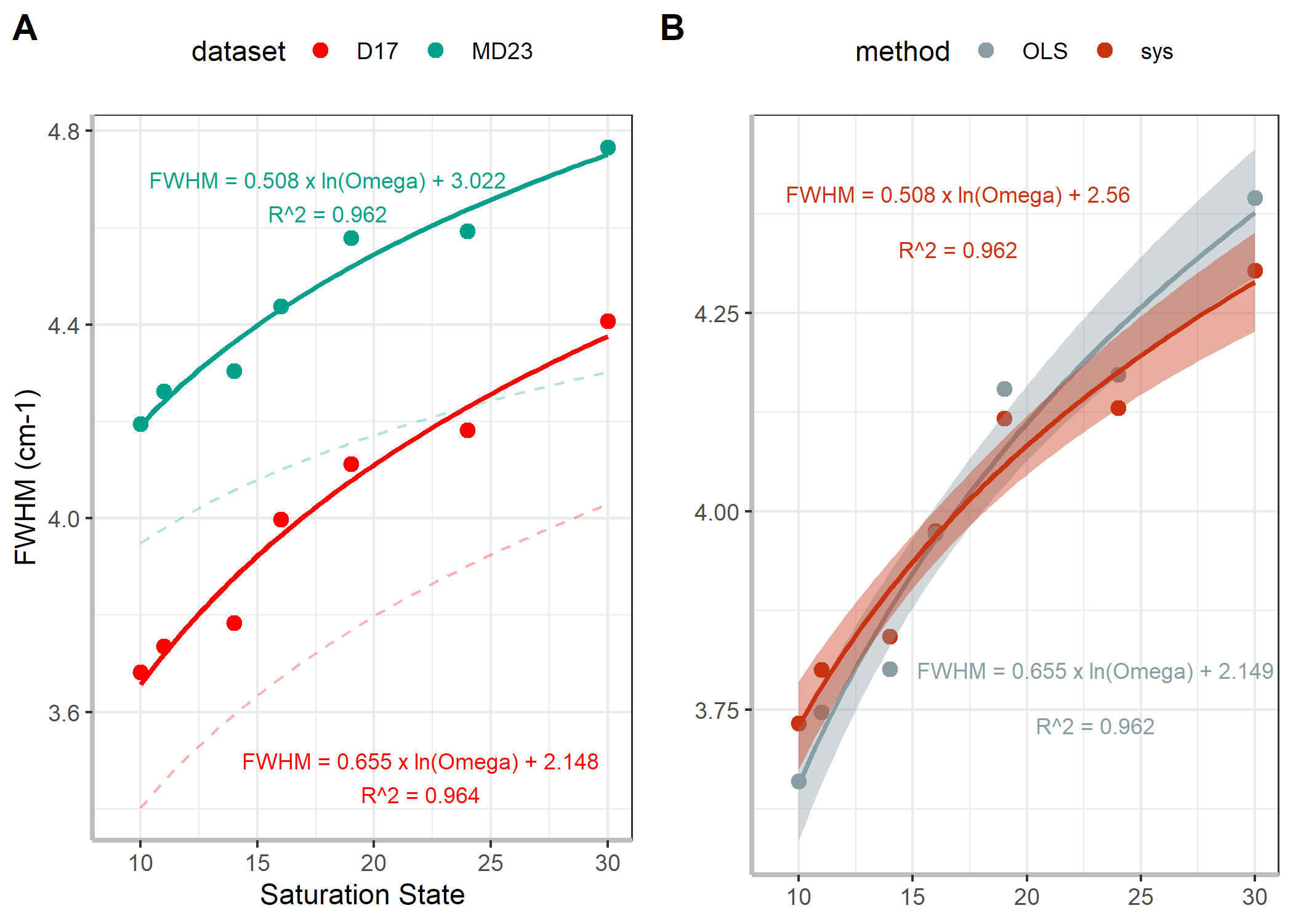
We can now build the two calibration curves for these datasets. I’ll also build 2 additional calibrations of the MD23 dataset, corrected to match the D17 dataset assuming a systematic error (subtract constant) and an OLS regression.
Figure 3. Logarithim calibration curves from A raw datasets and B corrected MD23 datasets
 So now we have four different calibration curves all generated from
abiogenic samples measured by D17 and MD23 analyzed with the Kiel
routine. These four calibration curves are distinct from the two
published calibration curves in D17 and MD23, which are:
- FWHM = $0.57 \times ln(omega) + 2.09, R^2 = 0.95$ (D17)
- FWHM = $0.321 \times ln(omega) + 3.21, R^2 = 0.95$ (MD23)
These two published curves are visualized in Figure 3A by the light, dashed lines. They have on average a smaller FWHM due to the different spectra analysis routines as discussed in the JCp-1 section above.
Ideally, I’d use the MD23 curve analyzed with the Kiel routine (solid blue in Figure 3A), since this is the most recently published calibration curve by DeCarlo and is generated from a spectrometer nearly identical to that in Dr. Prasad’s lab. However, this requires 2 stages of data manipulation to align (1: JCp-1 derived systematic error to align our measurements to D17 values and then 2: OLS/systematic error correction to MD23 values). Therefore, I will take a more conservative approach and align our data to DeCarlo et al. (2017) by subtracting 0.494 and then estimate the FWHM with, FWHM = 0.655 x ln(omega) + 2.148.
Since we are only comparing FWHM and estimated calcifying fluid omega between samples measured on the same spectrometer, this exercise doesn’t really matter too much. However, if we want to compare either of these values to other published datasets, then we will need to put some more thought into this.
Coral Analysis
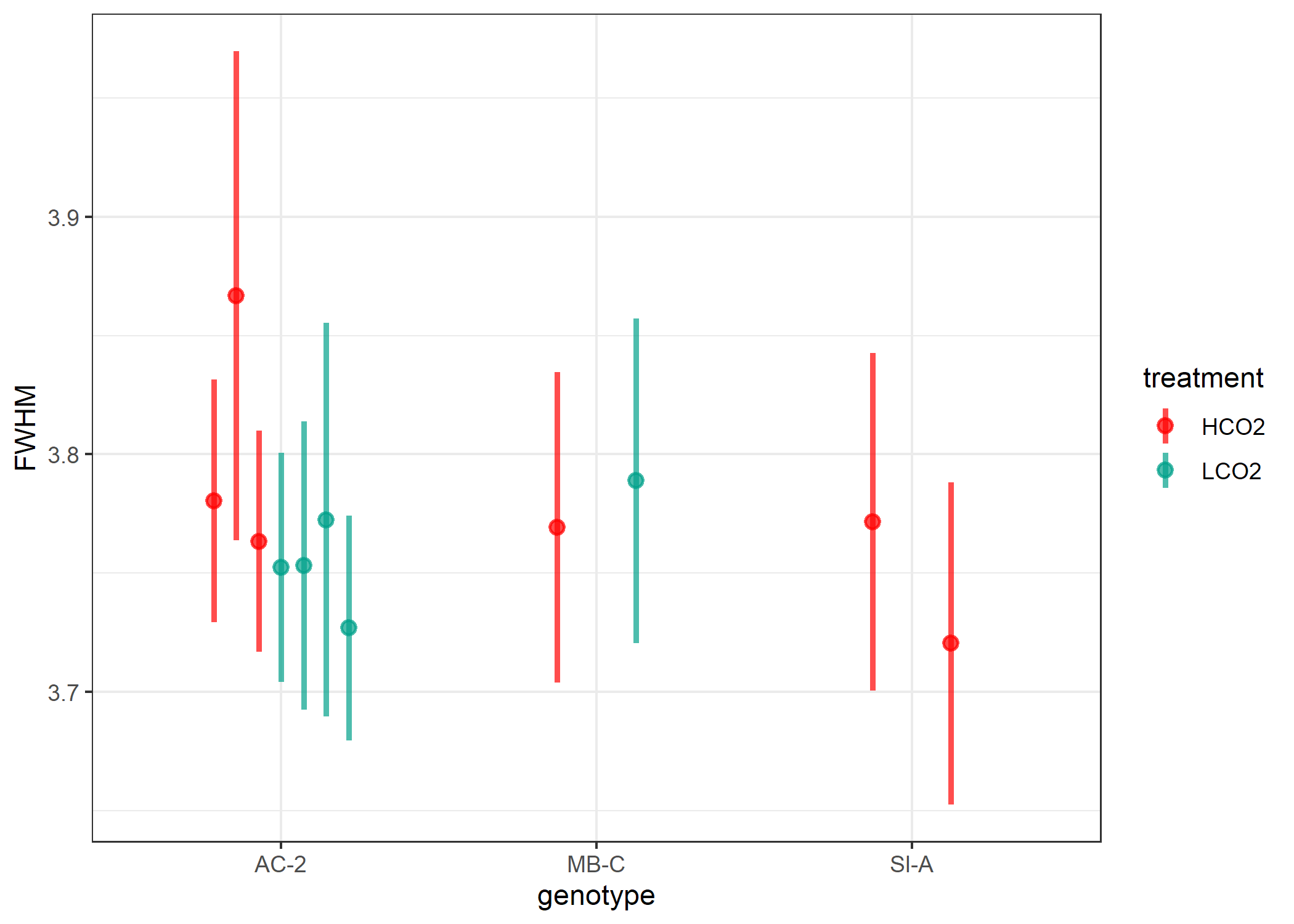
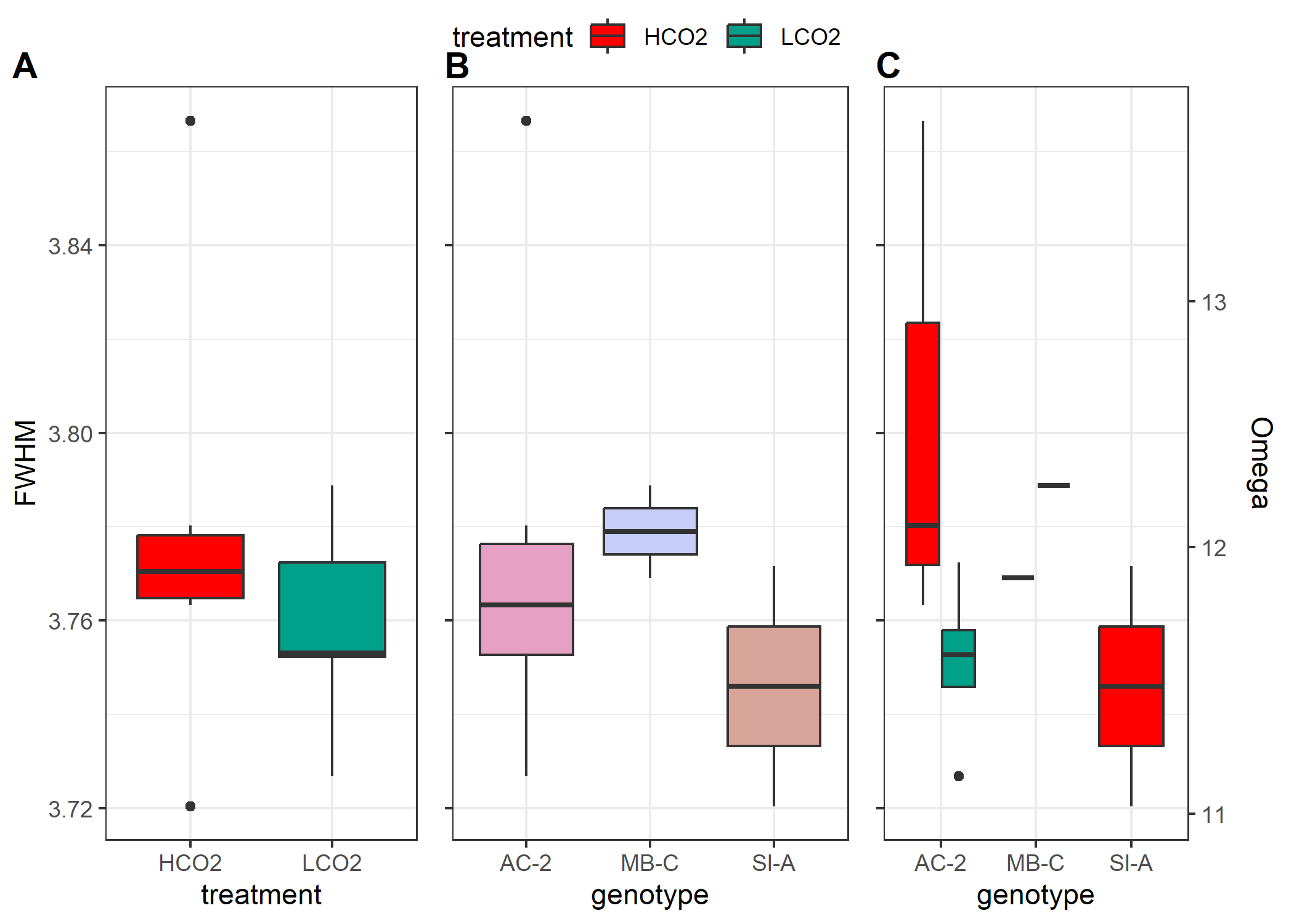 On first glance, this is not what I was expecting. First the FWHM of
these corals, and thereby the derived omega, do not have as much
variability as I was anticipating. Further, I was expecting the LCO2
corals to have a greater FWHM compared to the HCO2 corals. I chose these
11 samples as they had the greatest variability in $\delta^{11}B$ (proxy
for pH of the calcifying fluid), with the LCO2 having greater
$\delta^{11}B$ than HCO2 corals.
There are some limitations to this analysis. First, we only measured 11 samples and collected a single spectra on 10 haphazardly chosen grains for each sample. Some of the DeCarlo methods looked at 10-25 grains and collected 5-10 spectra per grain. I do not expect more spectra to drastically change our interpretation, but it may reduce our variability somewhat for each sample (shown below in Figure 4). Further, the uneven sample distribution combined with the one high measure of FWHM in an HCO2 Ac-2 sample is skewing our interpretation. All in all, I am planning to collect 3 spectra per grain with 25 grains per sample going forward. This will increase the measurement time on the Raman slightly, but should help and be worthwhile.
Figure 4. Significant variability exists for each grain, shown here is 1SD above and below the mean
Comparing the spectra
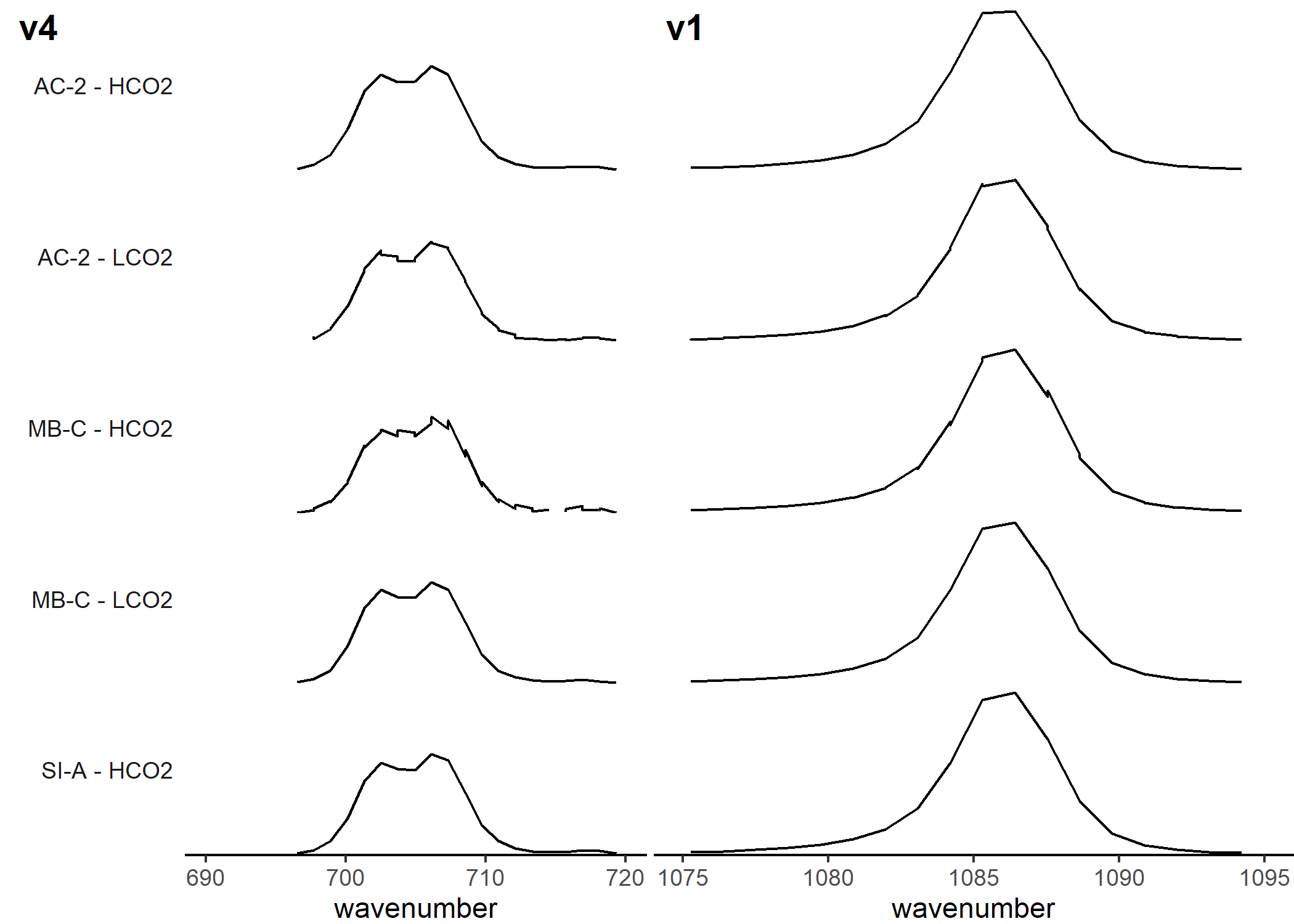
Here we are looking at an average spectra for each genotype-treatment combination to see if there are any visibly noticable differences other than v1 FWHM.From the v4 and v1 peak, we can’t really see anything too drastically different, and the v1 FWHM data from above corroborates this.
Figure 5. Mean generated spectra for each genotype-sample combination, centered at the v1 and v4 regions
Questions
The following are a bunch of remaining questions I have for this data, which I’d like to get a better handle of before measuring the remaining samples. These are the same questions I included in the email:
- After not observing burning of sample at low power, we set the laser intensity to 100% to maximize signal without saturating the spectra. The MD23 paper (with a similar if not identical Raman setup) used a laser intensity of 1% (from a 45mW source) and recorded peak intensity values much less than we were measuring. Their peak intensities were about 700 compared to ours at about 70,000. This two order of magnitude difference was reduced by SNV (z-score) normalizing the spectra, granting a normalized peak intensity of about 15 vs ours at about 18, highlighting the increased SNR of our spectra measured with a greater laser intensity. Are there any reasons to operate at a lower power besides not burning the sample, which we did not observe? From my understanding, the higher SNR should increase our ability to discern small-scale changes in peak widths. Is this correct?
- Similarly, prior literature used a 40x, 20x, and a 50x objective, while we used a 100x objective. Given the range of objectives used by different authors, I would not expect objective to alter the spectra. I’m assuming objective choice is function of grain size, with smaller grains needing greater magnification to properly focus. Does this make sense, or do you expect to see any differences based on objective alone?
- I have come across a single paper that attempts to standardize FWHM
across different machines by accounting for the spectral resolutions
of each individual spectrometer. DeCarlo et al. (2017) cites this
paper by Nasdala et al. (2001), which cites a German-language paper by Irmer
from 1985. However, DeCarlo does not use this method in any of his
subsequent papers and I have not come across this spectral
resolution standardizing equation in any other Raman resource I’ve
come across. This gives me the impression this practice is not
widely accepted or not widely used since Raman spectra are rarely compared between different
spectrometers. Their method is as follows,$b = b_s \times \sqrt{1-2(\frac{s}{b_s})^2}$,
where b is the corrected FWHM, $b_s$ is the measured FWHM, and s is the spectral
resolution of the Raman system.
- Have you come across any similar spectral resolution standardization technique before?
- Is spectral resolution just defined as the bins in the Raman shift, e.g. 1.14 $cm^{-1} from the Renishaw spectra$?
- Are there any steps in this analysis you find is lacking, not common practice, or needs more thought before measuring additional samples?