Langdon OA Corals
research 28 Jun 2022Overview
Here, I analyze the 11 coral skeletons grown under OA and ambient conditions. I first investigate the vertical extension and calcification data collected by the Langdon Lab, and then I look at the response of skeletal density to OA treatment. I further compare analyses at different thresholding, different scales of segmentation, and the different metrics I could standardize densities to facilitate “apples to apples” comparisons.
To remove genotype-specific variability from the analysis, a subset of 8 genetically distinct corals is selected with 4 corals each in the acidified group and the control group. The remaining 3 corals, all of genotype ‘P-Lirman’ and in the control group, are then compared to the other control corals to piece apart genotypic influence on skeletal bulk densities.
Linear Growth Analysis
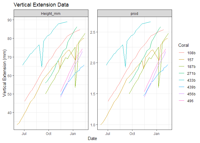
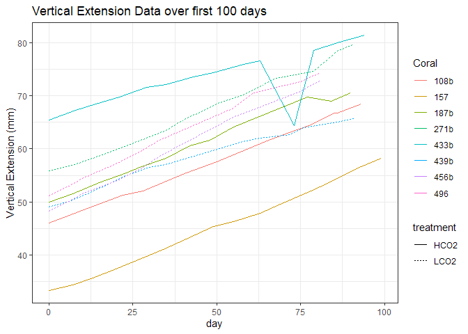
The sharp drop offs and increases in vertical extension are likely the artifact of a few erroneous data points. There were never 2 back to back data points like this, so the total growth, from initial to final is unaffeted.
Statistical Testing
Growth
## # A tibble: 2 x 4
##   treatment variable statistic     p
##   <chr>     <chr>        <dbl> <dbl>
## 1 HCO2      growth       0.998 0.995
## 2 LCO2      growth       0.980 0.902

## # A tibble: 1 x 5
##     df1   df2 statistic     p variable
##   <int> <int>     <dbl> <dbl> <chr>
## 1     1     6      1.32 0.294 growth
| .y. | group1 | group2 | n1 | n2 | statistic | df | p |
|---|---|---|---|---|---|---|---|
| growth | HCO2 | LCO2 | 4 | 4 | 2.083 | 6 | 0.082 |
| .y. | group1 | group2 | effsize | n1 | n2 | magnitude |
|---|---|---|---|---|---|---|
| growth | HCO2 | LCO2 | 1.473 | 4 | 4 | large |
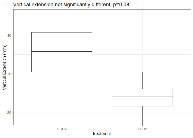
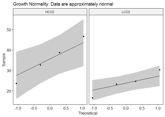
The mean growth in the HCO2 group was 35.43 mm (SD = 9.77mm), whereas the mean in LCO2 group was 23.69mm (SD = 5.63mm). A Student’s two-samples t-test showed that the difference was not statistically significant, t(6) = 2.083, p > 0.05, d = 1.473. Due to the small sample size, a type 2 error might be happening where we are accepting the null hypothesis. Further, the different number of days and times of the year when corals were observed obfuscates any conclusions.
Productivity
Using the productivity (growth standardized to initial size) metric from
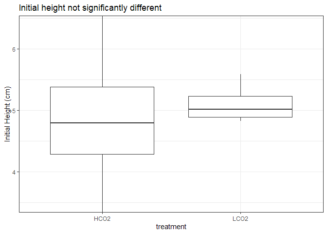
Lirman et al. 2014.
## # A tibble: 2 x 4
##   treatment variable     statistic     p
##   <chr>     <chr>            <dbl> <dbl>
## 1 HCO2      productivity     0.962 0.794
## 2 LCO2      productivity     0.978 0.890

## # A tibble: 1 x 5
##     df1   df2 statistic     p variable
##   <int> <int>     <dbl> <dbl> <chr>
## 1     1     6   0.00748 0.934 productivity
| .y. | group1 | group2 | n1 | n2 | statistic | df | p |
|---|---|---|---|---|---|---|---|
| prod | HCO2 | LCO2 | 4 | 4 | -1.125 | 6 | 0.304 |
| .y. | group1 | group2 | effsize | n1 | n2 | magnitude |
|---|---|---|---|---|---|---|
| prod | HCO2 | LCO2 | -0.796 | 4 | 4 | moderate |
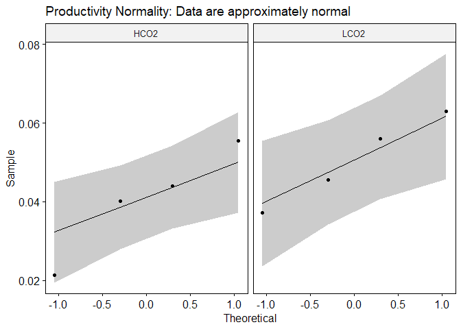
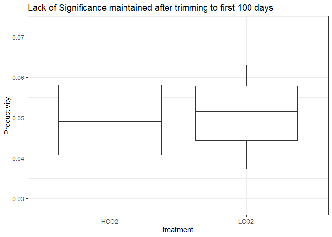
The mean productivity in the HCO2 group was 0.04 mm (SD = 0.01mm), whereas the mean in LCO2 group was 0.05mm (SD = 0.01mm). A Student’s two-samples t-test showed that the difference was not statistically significant, t(6) = -1.125, p > 0.05, d = -0.796.
Number of Days
| .y. | group1 | group2 | n1 | n2 | statistic | df | p |
|---|---|---|---|---|---|---|---|
| days | HCO2 | LCO2 | 4 | 4 | 4.154 | 3.905 | 0.015 |
| .y. | group1 | group2 | effsize | n1 | n2 | magnitude |
|---|---|---|---|---|---|---|
| days | HCO2 | LCO2 | 2.938 | 4 | 4 | large |
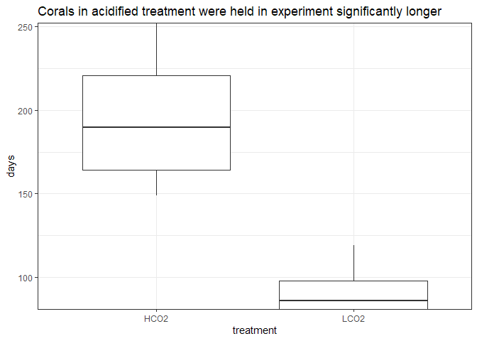
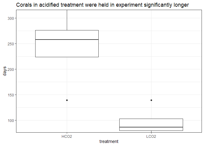
The mean days in experiment of the HCO2 group was 195 days (SD = 45.7), whereas the mean in LCO2 group was 93 days (SD = NA). A Welch’s two-samples t-test showed that the difference was statistically significant, t(3.91) = 4.15, p < 0.05, d = 2.938.
Due to the different number of days, I am trimming the observation of the OA corals to approximately equal the number of days of the control corals.
Calcification Analysis
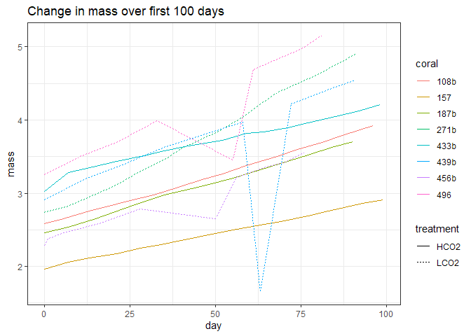
Calcification rates were determined by weekly measurements of buoyant weight. Mass gained during the experiment was standardized to initial mass.
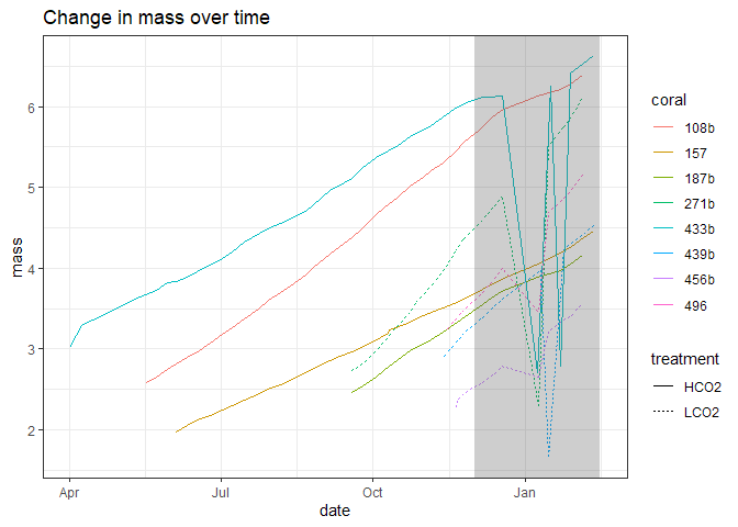
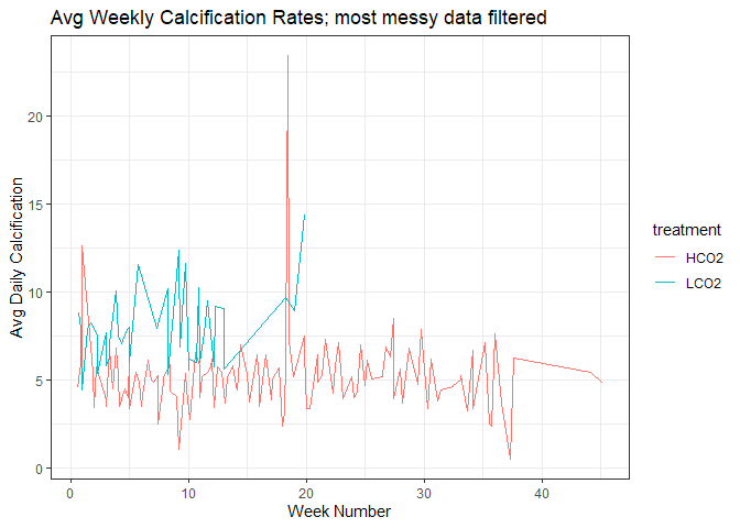
The data becomes a little messy between December and February near the end of the experiment with most of this mess centered around January 10th, 2022. Further, the different number of days and times of year as seen in linear extension data is present here and continues to muddle conclusions. Regardless, calcification is net positive by taking the difference in mass from the final and initial measurements.
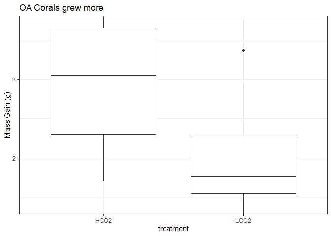
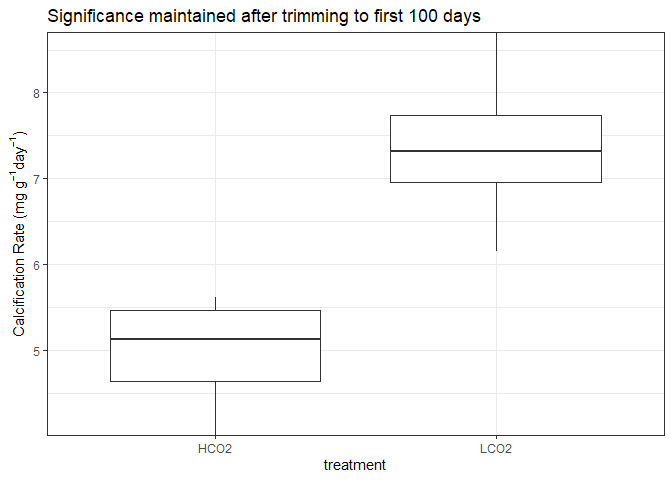
Due to the different number of days, I am trimming the observation of the OA corals to approximately equal the number of days of the control corals.
Statistical Testing
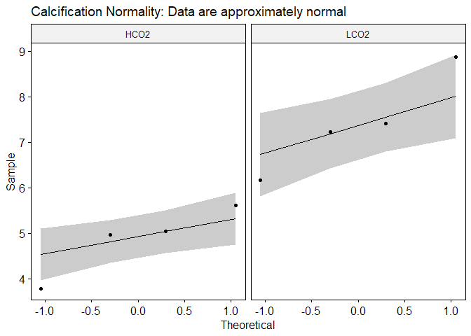
## # A tibble: 2 x 4
##   treatment variable statistic     p
##   <chr>     <chr>        <dbl> <dbl>
## 1 HCO2      G            0.909 0.479
## 2 LCO2      G            0.962 0.792

## # A tibble: 1 x 5
##     df1   df2 statistic     p variable
##   <int> <int>     <dbl> <dbl> <chr>
## 1     1     6     0.290 0.610 G
| .y. | group1 | group2 | n1 | n2 | statistic | df | p |
|---|---|---|---|---|---|---|---|
| G | HCO2 | LCO2 | 4 | 4 | -3.79 | 6 | 0.009 |
| .y. | group1 | group2 | effsize | n1 | n2 | magnitude |
|---|---|---|---|---|---|---|
| G | HCO2 | LCO2 | -2.68 | 4 | 4 | large |
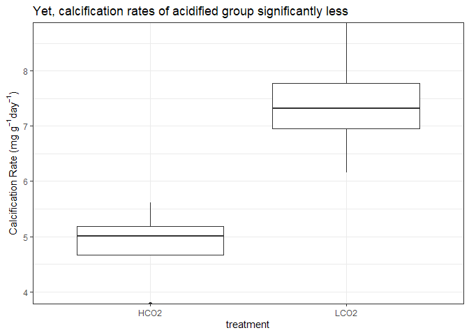
The mean calcification rate in the HCO2 group was 4.85 mg/g/day (SD = 0.77), whereas the mean in LCO2 group was 7.42 mg/g/day (SD = 1.12). A Student’s two-samples t-test showed that the difference was statistically significant, t(6) = -3.79, p < 0.01, d = -2.68.
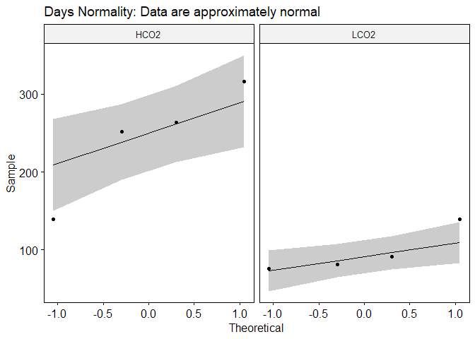
## # A tibble: 2 x 4
##   treatment variable statistic     p
##   <chr>     <chr>        <dbl> <dbl>
## 1 HCO2      days         0.917 0.521
## 2 LCO2      days         0.810 0.121

## # A tibble: 1 x 5
##     df1   df2 statistic     p variable
##   <int> <int>     <dbl> <dbl> <chr>
## 1     1     6     0.962 0.365 days
| .y. | group1 | group2 | n1 | n2 | statistic | df | p |
|---|---|---|---|---|---|---|---|
| days | HCO2 | LCO2 | 4 | 4 | 3.651 | 6 | 0.011 |
| .y. | group1 | group2 | effsize | n1 | n2 | magnitude |
|---|---|---|---|---|---|---|
| days | HCO2 | LCO2 | 2.582 | 4 | 4 | large |
The mean days in experiment of the HCO2 group was 242.5 days (SD = 74.44), whereas the mean in LCO2 group was 96.75 days (SD = 28.85). A Student’s two-samples t-test showed that the difference was statistically significant, t(6) = 3.65, p < 0.05, d = 2.582.
Growth Data Summarized
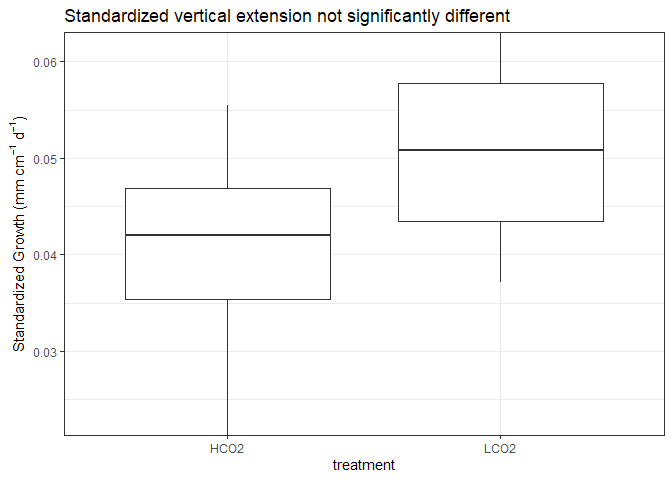
In summary, standardized vertical extension data was not signifcantly different among treatment groups. However, calcification rates were significantly different, with acidified groups having significantly less calcification rates. This falls in line with other OA experiments which observed a decreased in net calcification rates, but observed no differences in linear extension.
However, the length of observation was significantly different with control corals observed in the experiment significantly less than acidified treatment corals. This is critical for phenotypically plastic corals such as A. cervicornis (Kuffner et al. 2017), where the corals’ morphology and bulk density will be shaped by its environment over short amounts of time. Thus, the longer exposure of corals in lab conditions will artificially increase its bulk density compared to corals held in the lab over much shorter time frames. This is because nursery grown corals grow in the midwater column and are highly porous compared to corals grown in a lab which are affixed to a tag and held stationary in an aquarium. Over time, the density will increase in the lab relative to the nursery, and the amount of this density increase is directly proportional to time in the lab and any experimental conditions (acidified treatment). Since there is a difference in these two variables (length of time and control/treatment), we are unable to parse apart the relative significance of each of these factors, particularly with the small sample size present.
Skeletal Density Analysis
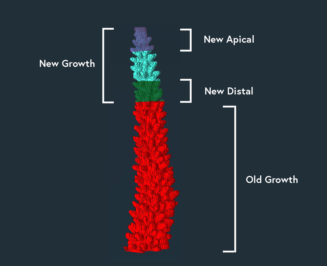
Skeletal density of the corals was measured by CT scanning with a Siemens Somatom Volume Zoom CT scanner at a resolution of 0.1mm scan − 1. The three dimensional reconstruction was digitally bisected using the software Amira (ThermoFischer Scientific) at the distance of new growth from the most distal slice of the apical branch. Materials were first assigned ‘Old Growth’ (red) and ‘New Growth’ (blue), where ‘Old Growth’ denotes the portion of the skeleton that was present at the beginning of the experiment and ‘New Growth’ denotes the portion of the skeleton that is grown under treatment conditions. The ‘New Growth’ section was then further segmented into ‘apical’ (purple) and ‘distal’ (green), where ‘apical’ and ‘distal’ denote 7.5mm sections of new growth. These standardized subsections permit additional analyses of the skeletal densities. Finally, ‘Old Growth’ and ‘New Growth’ were combined to do bulk scale analyses on the complete coral.
Because coral growth has vertical and lateral components, the ‘Old Growth’ material contains the initial skeleton and laterally grown calcium carbonate. However, we are unable to accurately parse apart these two growth forms in this material. Thus, ‘New Growth’, or the portion of the skeleton that grew above the maximum height of the initial skeleton, is the only section of the coral we can accurately analyze for treatment effect on skeletal density.
Bisected Slice = Distal Slice − [(Hf − Hi) * 10] where H is measured in mm, and slices represent 0.1mm of the skeleton’s reconstruction.
Then, holes were filled of the reconstruction to enclose the volume of the skeleton to be comparable with methods that determine skeletal density using the buoyant weight technique of wax sealed coral fragments. Finally, the mean brightness of the entire volume of new growth was converted to real-world skeletal density using aragonite density phantoms.
Two different material thresholds were selected for further comparison. The lab standard is to use -250, but I additionally tested -800 to prevent the clipping of low brightness data that may occur near the columella, apical tip, and the edge of the thecas. The result is the increased volume of the reconstruction and a slight increase in the brightness cumulative sum count, resulting in a overall reduction in average determined density. I compare the different values of the new growth at each of these thresholds in more depth below.
Old Growth v New Growth
| coral | treatment | Coral | NewGrowth | OldGrowth |
|---|---|---|---|---|
| 108b | HCO2 | 1.941 | 1.741 | 2.023 |
| 157 | HCO2 | 1.789 | 1.700 | 1.866 |
| 187b | HCO2 | 1.661 | 1.432 | 1.755 |
| 271b | LCO2 | 1.501 | 1.168 | 1.590 |
| 433b | HCO2 | 2.015 | 1.537 | 2.087 |
| 439b | LCO2 | 1.779 | 1.520 | 1.818 |
| 456b | LCO2 | 1.632 | 1.457 | 1.672 |
| 496 | LCO2 | 1.617 | 1.362 | 1.656 |

Across all materials, corals grown under LCO2 (control) are less dense than treatment corals. Further, New Growth is less dense than Old Growth which makes sense as the Old Growth contains the initial skeleton present at the beginning of the experiment with the addition of lateral thickening. Further, New Growth contains the fast growing apical branch which is less dense than the basal portion of the colony.
The decreased density in control corals compared to acidified corals is surprising, and does not agree with previous OA literature (Tambutte et al. 2015; Mollica et al. 2018). One interpretation is that the treatment group had significant effect on both the vertical extension and the lateral thickening of coral growth, and thus treatment effect is apparent in both the ‘New Growth’ and ‘Old Growth’ materials. As mentioned before, this was to be expected, however we cannot parse apart skeleton grown under treatment conditions in the Old Growth section. More likely, the differences in density is a factor of the amount of time held in the experiment, with corals held in the experiment longer have signifcantly more time to thicken the skeleton.
Correcting with calcification rates
If we assume that the rate of densification is equal to that of calcifiction, we can use the calcification rate, along with the final density of the new growth to compare corals.
Statistical Testing
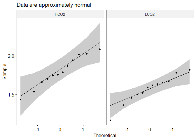
## # A tibble: 6 x 5
##   treatment material  variable statistic     p
##   <chr>     <chr>     <chr>        <dbl> <dbl>
## 1 HCO2      Coral     density      0.963 0.796
## 2 HCO2      NewGrowth density      0.923 0.555
## 3 HCO2      OldGrowth density      0.950 0.719
## 4 LCO2      Coral     density      0.960 0.782
## 5 LCO2      NewGrowth density      0.939 0.651
## 6 LCO2      OldGrowth density      0.916 0.512

## # A tibble: 3 x 6
##   material    df1   df2 statistic     p variable
##   <chr>     <int> <int>     <dbl> <dbl> <chr>
## 1 Coral         1     6    1.16   0.323 density
## 2 NewGrowth     1     6    0.0137 0.911 density
## 3 OldGrowth     1     6    1.95   0.212 density
| material | .y. | group1 | group2 | n1 | n2 | statistic | df | p |
|---|---|---|---|---|---|---|---|---|
| Coral | density | HCO2 | LCO2 | 4 | 4 | 2.248 | 6 | 0.066 |
| NewGrowth | density | HCO2 | LCO2 | 4 | 4 | 2.146 | 6 | 0.076 |
| OldGrowth | density | HCO2 | LCO2 | 4 | 4 | 2.783 | 6 | 0.032 |
| .y. | group1 | group2 | effsize | material | n1 | n2 | magnitude |
|---|---|---|---|---|---|---|---|
| density | HCO2 | LCO2 | 1.589 | Coral | 4 | 4 | large |
| density | HCO2 | LCO2 | 1.518 | NewGrowth | 4 | 4 | large |
| density | HCO2 | LCO2 | 1.968 | OldGrowth | 4 | 4 | large |
A Student’s two-samples t-test only showed statistically significant differences for the OldGrowth material, t(6) = 2.783, p < 0.05, d = 1.968. The New Growth material and the complete coral was just outside our significance threshold. There exist three interpretations: 1) The skeletons were significantly different prior to the experiment and the treatment did not alter the densities, or 2) the control treatment precluded the lateral thickening of the corals while maintaining the linear extension as evidenced by the similiar producitivty values and densities of new growth, yet old growth (existing + latral thickening) was diminished. This interpretation would be characteristic of growth patterns seen in the literature for acidified groups, and not ambient control groups. Or 3) the increase in density (although only significant at the old growth) is a factor of the length of time in the treatment with the theory explained above. Again, it is important to place these interpretations alongside the small samples size.
Thresholding Differences
As mentioned in the overview, the lab standard for analysis of coral CT Scans is to set the lower threshold limit at -250. This clips some brightness data and shrinks the calculated volume of the reconstruction with the benefit of definitively selecting coral material only and not air or other non-coral material. Since we are exploring low density growth patterns in a controlled experiment, I sought to forgoe the benefits of the conservative thresholding and employed a liberal thresholding of -800.
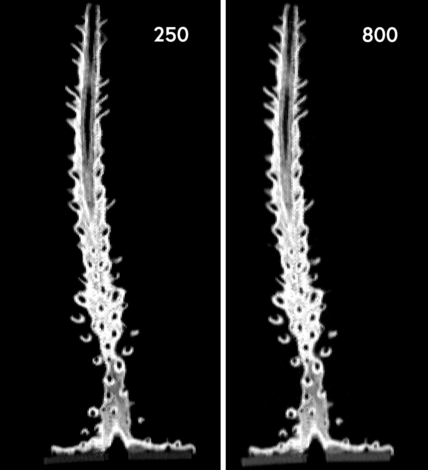
Here, I am comparing the different determinations of the two settings. In the image below you can see two identical slices at the different thresholding limits. It is barely noticeable at this scale to the naked eye, but there is slightly more material included in the -800 thresholding with the width of the columella being less than the width of the columella in the -250. Thus, the increased thresholding permits the region of interest (skeletal material) to penetrate into this low density portion of the skeleton.
| metric | mean | sd |
|---|---|---|
| density | -14.0 | 5.0 |
| volume | 17.2 | 7.1 |
On average, the -800 thresholded reconstruction has a volume 17.2% greater than the -250 reconstruction by including more low density material, resulting in an average determined density 14% less than the -250 reconstruction. This lines up well with our theory of segmentation. Certainly, a -250 reconstruction should not be compared to a -800 reconstruction, but the variability within each group is fairly uniform.
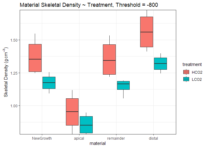
With that in mind, I will proceed with the -800 reconstruction and subsection out materials in the New Growth material. These densities will be different than the New Growth shown above and will only be compared to other -800 reconstructions.
Subsectioning New Growth
Statistical Testing
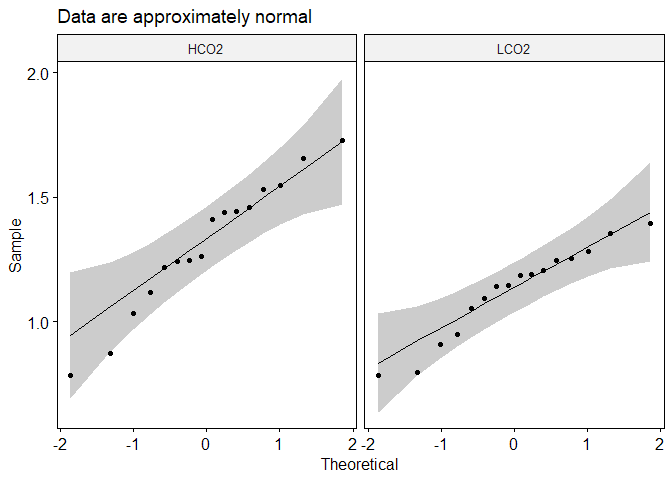
## # A tibble: 8 x 5
##   treatment material  variable statistic     p
##   <chr>     <fct>     <chr>        <dbl> <dbl>
## 1 HCO2      NewGrowth density      0.881 0.343
## 2 HCO2      apical    density      0.959 0.775
## 3 HCO2      remainder density      0.879 0.333
## 4 HCO2      distal    density      0.897 0.415
## 5 LCO2      NewGrowth density      0.982 0.911
## 6 LCO2      apical    density      0.864 0.273
## 7 LCO2      remainder density      0.841 0.198
## 8 LCO2      distal    density      0.963 0.800

## # A tibble: 4 x 6
##   material    df1   df2 statistic      p variable
##   <fct>     <int> <int>     <dbl>  <dbl> <chr>
## 1 NewGrowth     1     6      4.81 0.0708 density
## 2 apical        1     6      3.93 0.0948 density
## 3 remainder     1     6      7.54 0.0335 density
## 4 distal        1     6     12.3  0.0127 density
| material | .y. | group1 | group2 | n1 | n2 | statistic | df | p |
|---|---|---|---|---|---|---|---|---|
| NewGrowth | density | HCO2 | LCO2 | 4 | 4 | 2.486 | 4.354 | 0.063 |
| apical | density | HCO2 | LCO2 | 4 | 4 | 1.087 | 4.614 | 0.330 |
| remainder | density | HCO2 | LCO2 | 4 | 4 | 2.608 | 3.988 | 0.060 |
| distal | density | HCO2 | LCO2 | 4 | 4 | 2.914 | 4.132 | 0.042 |
| .y. | group1 | group2 | effsize | material | n1 | n2 | magnitude |
|---|---|---|---|---|---|---|---|
| density | HCO2 | LCO2 | 1.758 | NewGrowth | 4 | 4 | large |
| density | HCO2 | LCO2 | 0.769 | apical | 4 | 4 | moderate |
| density | HCO2 | LCO2 | 1.844 | remainder | 4 | 4 | large |
| density | HCO2 | LCO2 | 2.061 | distal | 4 | 4 | large |
A Welch’s two-sample t-test only showed statistically significant differences for the distal material, t(4.13) = 2.91, p < 0.05, d = 2.061. The remainder material and the new growth material analyzed as a whole was just outside our significance threshold, and the apical matrial was highly variable and not significantly different, p > 0.33. Thus, from the distal to apical regions of the new growth, variability within treatment group increases and the ability to detect treatment effect decreases. This falls in line with our understanding of coral growth in the highly variable, fast growing apical tips. Further, this closely aligns with the prior analysis of new growth v old growth, where new growth was not signifcantly different between control and treatment, but old growth was different between the groups. Finally, the trend of denser skeletons in the control group compared to the treatment group aligns with the previous analysis with the likely cause being the amount of days grown in the lab.
Estimating Mass Gain
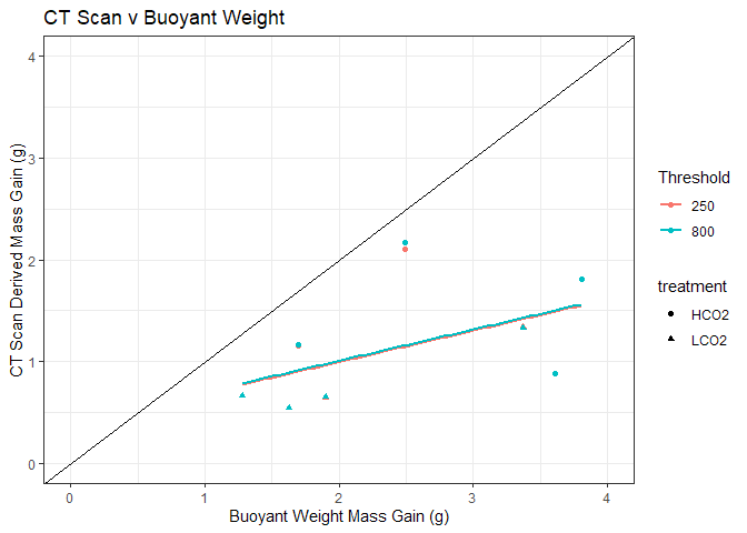
Calcification can also be determined by multiplying the volume of the new growth section by the average density of this material. We can compare this calculated mass to to the buoyant weight data. We can further see which thresholding has a better fit with the buoyant weight data to add to our comparison of thesholding differnces.
##
## Call:
## lm(formula = calcMass ~ newMass, data = newMass)
##
## Residuals:
##     Min      1Q  Median      3Q     Max
## -0.6187 -0.3328 -0.1018  0.2494  1.0180
##
## Coefficients:
##             Estimate Std. Error t value Pr(>|t|)
## (Intercept)   0.3837     0.3522   1.089   0.2943
## newMass       0.3078     0.1332   2.312   0.0365 *
## ---
## Signif. codes:  0 '***' 0.001 '**' 0.01 '*' 0.05 '.' 0.1 ' ' 1
##
## Residual standard error: 0.4958 on 14 degrees of freedom
## Multiple R-squared:  0.2762, Adjusted R-squared:  0.2246
## F-statistic: 5.344 on 1 and 14 DF,  p-value: 0.03653
Multiplying ct scan density and volume underestimates the derived mass gain as compared to buoyant weight data. To some extent, this was to be expected. Calcification takes place not only in the new growth, but also in the lateral thickening of the old growth section which was not included in the CT Scan derived mass. Except for one data point which nearly has a 1:1 relationship (85%), the other 7 corals have their calculated mass gain at about 43% of mass gain as measured by buoyant weight.
There was no observable difference in calculation of mass between the 250 and 800 thresholded reconstructions. Again, this was to be expected as calculated gain in mass is the product of volume and density. The two different reconstructions have nearly equal and opposite determinations of each, balacing out the equation and resulting in nearly similar mass: vol250 < vol800, ρ250 > ρ800, mass250 ≈ mass800
Standardization Metrics
Number of Days in Treatment
Due to the different number of days in treatment and control groups, I am tempted to standardize the density of the corals to its number of days in treatment. This should standardize the number of days an individual coral was able to fill in its skeleton in the laboratory at its specified treatment.
There are multiple caveats: 1) we have already sectoned out the new growth in the treatment, 2) units will be expressed in density/days which is an arbitrary unit without a real-world meaning, and 3) the range of the days are fairly large (>150 days difference between group means), and the data may just be incomparable.
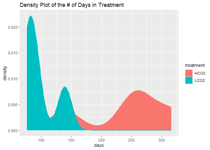
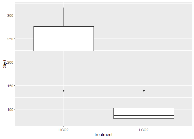
Nevertheless, here is the data standardized to the number of days in treatment.
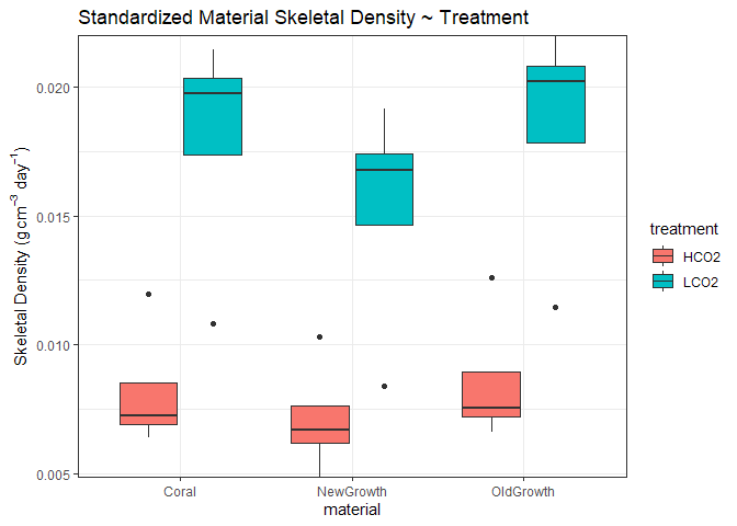
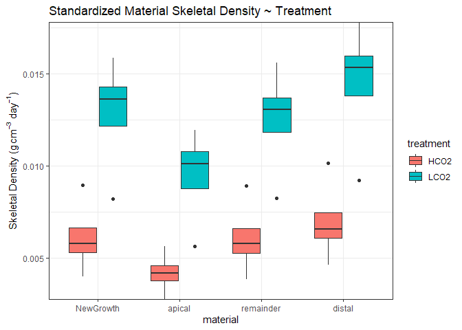
Now, there are significant differences with LCO2 corals being denser than OA corals. However, the differences across sectioned materials and different thresholds is nearly uniform, suggesting that the driving force is not the difference in densities of each material (as shown above in the normal data and backed with theory), but rather the standardizing metric. Further, the differences reflect the reciprocal of the boxplot above, underscoring the difference in number of days is driving the observed differences.
I conclude that standardizing to the number of days in treatment is not an appropriate metric.
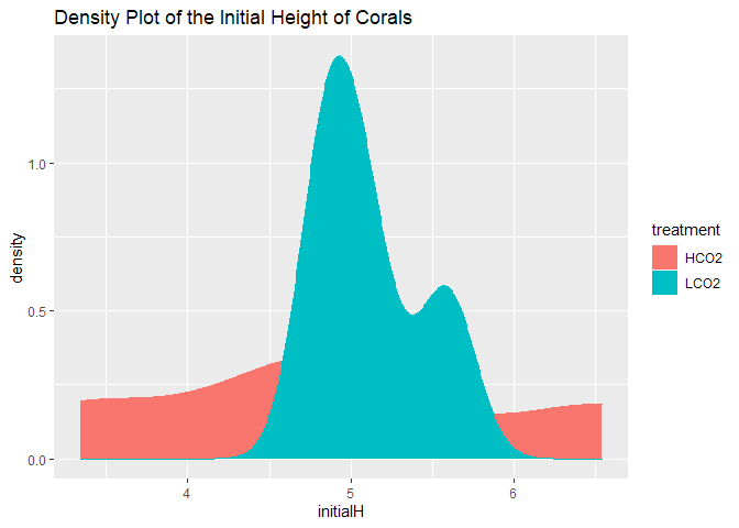
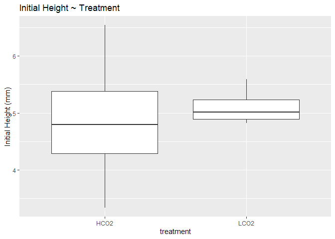
Initial Height of Coral
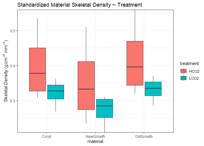
Just as we standardized total vertical extension to initial height of the coral, we can standardize density of the coral to its initial height. However, this shares many of the same caveats from above, namely that density/height is an arbitrary, potentially meaningless unit.

## # A tibble: 3 x 9
##   material  .y.     group1 group2    n1    n2 statistic    df     p
## * <chr>     <chr>   <chr>  <chr>  <int> <int>     <dbl> <dbl> <dbl>
## 1 Coral     density HCO2   LCO2       4     4      1.42     6 0.206
## 2 NewGrowth density HCO2   LCO2       4     4      1.25     6 0.257
## 3 OldGrowth density HCO2   LCO2       4     4      1.52     6 0.18

## # A tibble: 4 x 9
##   material  .y.     group1 group2    n1    n2 statistic    df     p
## * <fct>     <chr>   <chr>  <chr>  <int> <int>     <dbl> <dbl> <dbl>
## 1 NewGrowth density HCO2   LCO2       4     4     1.34      6 0.229
## 2 apical    density HCO2   LCO2       4     4     0.979     6 0.366
## 3 remainder density HCO2   LCO2       4     4     1.38      6 0.216
## 4 distal    density HCO2   LCO2       4     4     1.39      6 0.215
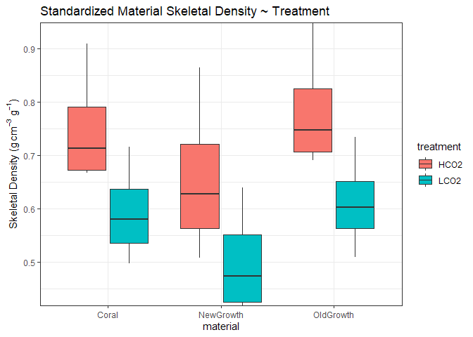
Here, we see the same initial pattern with OA corals generally more dense than control corals. However, significant differences between any material has been lost. HCO2 corals had more variable initial height but the mean value did not differ significantly.
Initial Mass of Coral
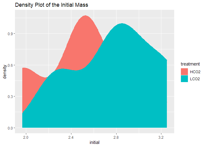
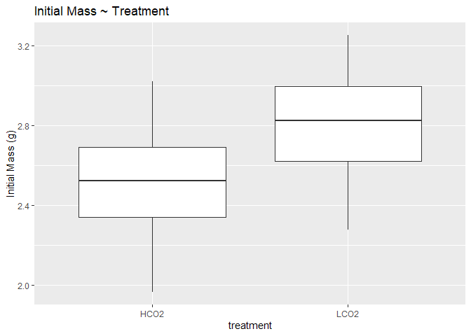
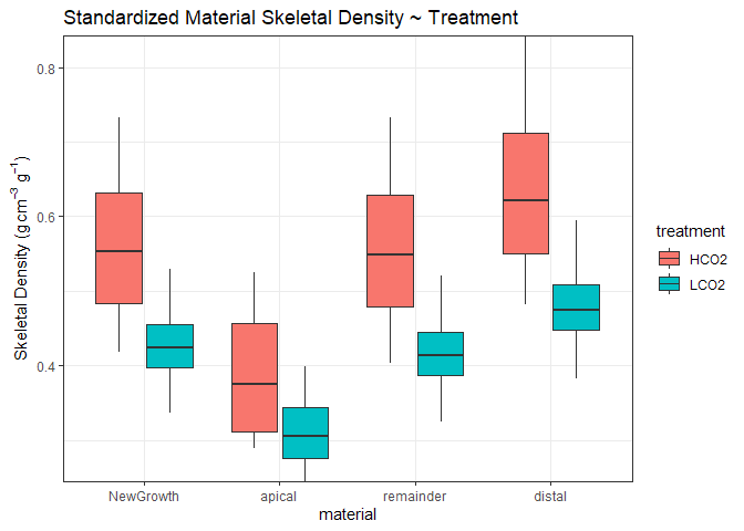
Same concept, but using initial mass to standardize just as we did for calcification.
## # A tibble: 3 x 9
##   material  .y.     group1 group2    n1    n2 statistic    df      p
## * <chr>     <chr>   <chr>  <chr>  <int> <int>     <dbl> <dbl>  <dbl>
## 1 Coral     density HCO2   LCO2       4     4      2.14     6 0.076
## 2 NewGrowth density HCO2   LCO2       4     4      1.68     6 0.145
## 3 OldGrowth density HCO2   LCO2       4     4      2.29     6 0.0622

## # A tibble: 4 x 9
##   material  .y.     group1 group2    n1    n2 statistic    df     p
## * <fct>     <chr>   <chr>  <chr>  <int> <int>     <dbl> <dbl> <dbl>
## 1 NewGrowth density HCO2   LCO2       4     4      1.73     6 0.134
## 2 apical    density HCO2   LCO2       4     4      1.22     6 0.267
## 3 remainder density HCO2   LCO2       4     4      1.74     6 0.132
## 4 distal    density HCO2   LCO2       4     4      1.81     6 0.12
Again, the same initial pattern with significant differences between any material lost.
Genotype Variability
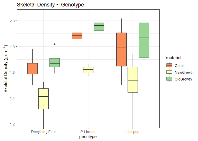
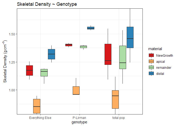
Finally, it is important to compare the variability of the population to the variability of a genoype within that population to begin to understand genotype-specific sensitivities. Here, I compare 3 ramets of P-Lirman grown under LCO2 conditions and compare it to all LCO2 corals
## # A tibble: 3 x 6
## # Groups:   material [3]
##   material  threshold statistic p.value parameter method
##   <chr>         <dbl>     <dbl>   <dbl>     <dbl> <chr>
## 1 Coral           250      2.70   0.260         2 Bartlett test of homogeneity ~
## 2 NewGrowth       250      2.65   0.266         2 Bartlett test of homogeneity ~
## 3 OldGrowth       250      2.55   0.279         2 Bartlett test of homogeneity ~
##   Tukey multiple comparisons of means
##     95% family-wise confidence level
##
## Fit: aov(formula = density ~ genotype, data = .)
##
## $genotype
##                                  diff          lwr        upr     p adj
## P-Lirman-Everything Else   0.25151849  0.040800773 0.46223621 0.0156768
## total pop-Everything Else  0.15266046 -0.008427085 0.31374800 0.0666405
## total pop-P-Lirman        -0.09885804 -0.278558712 0.08084264 0.3864274
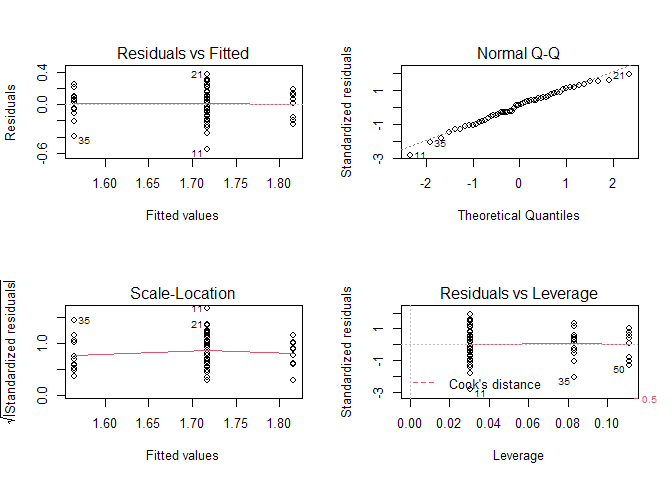
From this data, there are significant differences of skeletal density among the genotype P-Lirman as compared to the rest of the population (p<0.05). However, when grouped together, there is no difference of P-Lirman (p=0.386). This could suggest that there is significant genotypic variability, shown here with only 3 corals compared to the 8 other corals. Certainly, more analysis needs to be done.